

Biquadratic interpolation with independent sample weights
- Thomas Deliot
- 30 mars 2020
- 5 min de lecture

Dernière mise à jour : 14 oct. 2024
This thread on StackExchange asks a great question: why is quadratic interpolation so rarely used, especially in computer graphics ? Linear interpolation provides fast, low quality results using 2 samples, while cubic interpolation provides slower, higher quality results with 4 samples. It seems that quadratic interpolation, with 3 samples, would offer more control on cost vs quality, especially in the 2D case at 4 vs 9 vs 16 samples.
It can be a useful tool where one can't afford the 4*4 samples for smooth bicubic interpolation but bilinear isn't good enough. It is especially useful when the 3*3 neighbourhood values are already available due to some other process, as can often be the case in post-processing. And while bicubic interpolation can be obtained with only 4 (bilinear filtered) texture samples, this cannot be used when one needs to dynamically modulate the individual weights of each sample, such as is the case for bilateral or depth-aware upsampling filters.
I happened to be precisely in that case when working on volumetric cloud depth-aware upsampling. Having my 3*3 neighbourhood values readily available, I found after a quick search no way to use them to their full advantage for interpolation, having to either fallback to bilinear with low quality, or to bicubic with more sampling. I wondered why and started trying it out myself when I quickly realized the reason : the symmetry of the problem didn't seem to allow it.
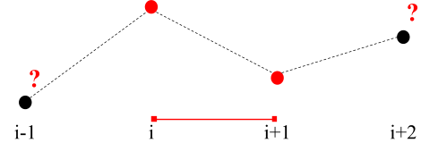
When interpolating at a position between two values on a 1D grid, it's straightforward to either take the 2 or 4 neighbouring control points around it and interpolate:

Linear and cubic interpolation
But if you want to take 3, which do you choose ? You get an additional value on either the left or the right, and you end up not centered around the interpolation interval anymore:
Alain Brobecker details a simple fix to this issue on his post about quadratic interpolation. Basically shift the problem half a unit to the left and use two new virtual control points, created by linearly interpolating the real ones. Note this means the curve no longer passes through the control points of your data set, but through the virtual control points:
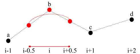
Quadratic interpolation
Summarizing Alain’s algorithm into a single equation, we can compute this interpolation with :
y = ((a+b)/2) + (2 * (b - (a+b)/2) * x) + (((b+c)/2 - 2b + (a+b)/2) * x²)
Where x is the local interpolation coordinate varying from 0 to 1 across the [ i-0.5 ; i+0.5 ] interpolation interval. Apply the same process to the next intervals and you get a C1 continuous quadratic interpolation of the data set, with a continuous derivative.
Now we can extend this to biquadratic interpolation, following the regular 1D to 2D scheme used to go from linear to bilinear and cubic to bicubic. We get the biquadratic algorithm by interpolating quadratically three times along one coordinate, and one last time along the other:
x1 = quadratic(a, b, c, x)
x2 = quadratic(d, e, f, x)
x3 = quadratic(g, h, i, x)
z = quadratic(x1, x2, x3, y)
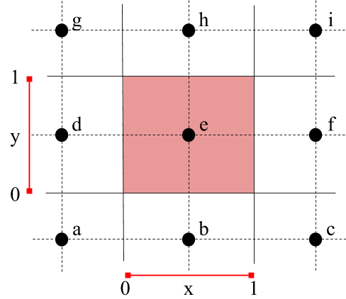
Using the following layout of control points and local (x, y) coordinates. This is a handy setup: it requires using the half-texel offset to correctly align the pixel values with their pixel centers, which should be done anyway. There's a much better visualization of this thanks to @paniq on shadertoy.
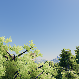
Next is a comparison between bilinear, biquadratic and bicubic using upsampled volumetric clouds as an example. In this setup, biquadratic interpolation achieves largely similar results to bicubic with only the 3x3 neighbouring values I already had available, saving me 7 additional samples.

Bilinear vs biquadratic vs bicubic upsampling
However, what I needed was a depth-aware upsampling filter. This adds another constraint for the interpolation scheme: separate weights for each control points. We need the biquadratic upsampling to be expressible in terms of a single equation: a weighted sum of the control points. In this form, each control point is only weighted by polynomials of x and y. If you then normalize this weight sum, this allows dynamically modulating each sample's weight.
To achieve this, we can first simplify the 1D quadratic equation into the form we want:
y = ((a+b)/2) + (2 * (b - (a+b)/2) * x) + (((b+c)/2 - 2b + (a+b)/2) * x²)
→ y = a(0.5 - x + 0.5x²) + b(0.5 + x - x²) + c(0.5x²)
Plugging this into the 2D sampling pattern gives :
abc = a(0.5 - x + 0.5x²) + b(0.5 + x - x²) + c(0.5x²)
def = d(0.5 - x + 0.5x²) + e(0.5 + x - x²) + f(0.5x²)
ijk = i(0.5 - x + 0.5x²) + j(0.5 + x - x²) + k(0.5x²)
z = abc(0.5 - y + 0.5y²) + def(0.5 + y - y²) + ijk(0.5y²)
Which can be developed into our desired form. Note that since this is a separable filter, many computations are reusable:
z = a(0.25 * (x - 1)² * (y - 1)²)
+ b(0.25 * -(2x² - 2x - 1) * (y - 1)²)
+ c(0.25 * x² * (y - 1)²)
+ d(0.25 * (x - 1)² * -(2y² - 2y - 1))
+ e(0.25 * -(2x² - 2x - 1) * -(2y² - 2y - 1))
+ f(0.25 * x² * -(2y² - 2y - 1))
+ g(0.25 * (x - 1)² * y²)
+ h(0.25 * -(2x² - 2x - 1) * y²)
+ i(0.25 * x² * y²)
This allows using smooth biquadratic upsampling in a depth-aware fashion, with discardable invalid samples:
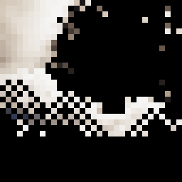
High-res scene and low-res volume buffer to splat in the scene. We only want to use the valid samples while splatting in the gaps between leaves.
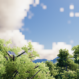
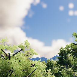
Bilinear vs Biquadratic depth-aware upsampling
Additional analysis
It was brought to my intention that this scheme for quadratic interpolation introduces a significant low-pass effect. This is absolutely correct, and brought me to do some plotting to look at its actual produced results. The Desmos graph is available here and also shows the derivatives of both the quadratic and cubic segments, with C1 and C2 continuity respectively.

Linear (red), quadratic (blue) and cubic (green) interpolation of an alternating signal
In the worst case scenario (an alternating signal), using quadratic interpolation introduces a 50% loss of contrast that linear and cubic do not suffer from, with resulting values ranging from 0.25 to 0.75 on the orginal 0 to 1 signal.
This is due to the fact that this quadratic interpolation scheme isn't actually an interpolating scheme, as it does not pass through the original values of the dataset. It is rather an interpolating scheme of the average virtual half-points, and only an approximating scheme of the real control points, always contained inside the boundaries of the polygon they form and pulled towards them.
It is also equivalent to the Corner Cutting subdivision scheme (thanks to Wojciech Jarosz for pointing it out!).
Commentaires